Put the program on a timeline
Read this line without running it:
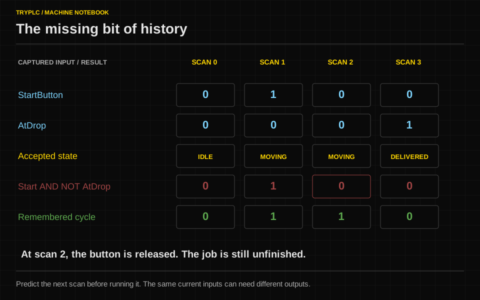
Q_Belt := StartButton AND NOT AtDrop;The line is valid. It also fails the one-carton contract. Syntax checking cannot tell you that Start is supposed to be a momentary request. The missing information only appears when you give the program an input history.
Three passes, with a deliberate boundary between them
On paper, divide one program evaluation into events and time, state decisions, and output assignment. This is a project organization choice, not a claim that every PLC has exactly three execution phases internally.
| Our program pass | Read | Write | Question answered |
|---|---|---|---|
| Events and time | Captured inputs and previous values | Edges and timer results | What newly happened, and what waited too long? |
| State decision | Current state, events, permissions, timer results | One next state | What work is now active? |
| Output assignment | Updated state and continuous permissions | Q_Belt once | What request may leave the controller? |
Use a separate NextState while making the decision. Assign it to State after the state selection finishes. Then calculate the output from that updated state. A newly accepted move can request the belt in the same program evaluation; an interruption can remove it in that evaluation. The physical output module still has its own update timing.
If you assign Q_Belt before changing State, you have chosen a different timing relationship. It may introduce an extra evaluation of delay. That is not automatically wrong, but it must be deliberate and reflected in the tests. “The lines are all there” is not enough; order is part of the behavior.
A trace you should be able to explain aloud
At the beginning of a moving scan, suppose Stop is TRUE and AtDrop is TRUE. The event pass captures those facts. The decision pass selects INTERRUPTED because the agreed priority puts Stop first. The output pass observes that the updated state is not MOVING and that Stop is active, so Q_Belt is FALSE. The trace should preserve the simultaneous facts; recording only the final state loses the reason for the decision.
Now imagine Start goes TRUE just after the input image is captured. A program using that captured image does not see the new press in the current evaluation. It may see it in the next one. A pulse shorter than the acquisition interval can be missed entirely. Use the actual module, filter and task timing when you need to guarantee capture.
The machine moves between observations
A PLC program usually returns to the same logic repeatedly. It does not wait inside a line of code while a carton travels. It observes, makes decisions, updates commands, and comes back later. Understanding that repetition removes many mysteries: why a button press is counted several times, why one instruction sees a new value and another sees an old one, and why a short sensor pulse can disappear entirely.
For the examples in this chapter, use a deliberately simple execution model. One cyclic task takes an input snapshot, executes its program in order, and publishes the resulting output commands. The next invocation repeats the process. Variables belonging to the program retain their working values between invocations unless the program changes them or initialization occurs.
That is our model, not a universal description of every controller's I/O scheduler. Actual systems may update remote I/O asynchronously, use several tasks, or provide direct peripheral access. Learn the simple model, then check where your target differs.
Walk through statements, not intentions
Suppose this excerpt executes once each scan. All three variables are Boolean, and Request begins false.
SeenBefore := Request;
Request := StartButton;
SeenAfter := Request;
When the sampled StartButton first becomes true, SeenBefore receives the old false value. The assignment changes Request immediately in program memory. SeenAfter then receives true. Nothing about the program's repeated execution makes those statements simultaneous.
| Scan | Sampled StartButton | Request at entry | SeenBefore at exit | SeenAfter at exit |
|---|---|---|---|---|
| 1 | False | False | False | False |
| 2 | True | False | False | True |
| 3 | True | True | True | True |
| 4 | False | True | True | False |
This is why “I assigned it somewhere in the program” is not enough. The assignment must happen before the consumer that needs the new value, or the design must intentionally use the previous value.
A physical output and its command are not the same clock
Under our teaching model, writing ConveyorCmd := TRUE changes the program's command variable during execution. The output transfer happens at the configured update point. A later statement may change the command again before that transfer.
ConveyorCmd := StartButton;
ConveyorCmd := FALSE;
The final command is false on every scan. The first line is not a brief, reliable motor pulse. With buffered output updates, the physical output may never see it. With direct writes or another task involved, behaviour could differ again. Either way, the code is a poor expression of intent.
Use one clear owner for an output. Other routines may calculate requests and restrictions; the owner combines them and writes the command. This makes the final result explainable without searching for the last of several competing assignments.
For a concrete manufacturer example, Siemens documents S7-1200 V20's normal cycle as output transfer, input acquisition, and program execution, with interrupts and communication also considered. Its process image gives the program a consistent set of sampled inputs for the relevant cycle. The location chosen as the “start” of a repeating cycle therefore matters when reading a timing diagram. Siemens scan-cycle description.
Estimate response time as a chain
Imagine an idealized task with an exactly 10 ms period. A sensor changes 1 ms after an input snapshot. The program does not observe it for another 9 ms. If program execution and output transfer then take 2 ms, the command reaches the modeled output 11 ms after the physical change.
That is not yet actuator response. Add sensor response, input filtering, network and module update delays, output switching, drive response, and mechanical motion as applicable. Use measured or specified bounds for the actual system. A fast average scan time does not establish a worst-case machine response.
Now let the sensor pulse last only 3 ms, entirely between snapshots. The task sees false before and false afterward. No clever rising-edge instruction can recover the missing pulse. You need a signal acquisition arrangement suited to the event: suitable filtering, a faster task and I/O update, pulse capture, a hardware counter, or another appropriate mechanism.
Tasks add another layer of order
A task is an execution schedule for program work. A slow monitoring task and a fast control task may access shared information at different times. If both write the same command or state, source-code order alone no longer tells the whole story. Priorities, preemption, update boundaries, and data consistency now matter.
Begin with one owner for each piece of state. Pass requests or snapshots between tasks using the target platform's supported mechanisms when multiple tasks are necessary. Do not add a fast task merely because a number looks more professional. It consumes processing capacity and can complicate the timing of everything around it.
Watchdog supervision detects execution that exceeds configured limits; it is not a substitute for bounding your work. A loop that waits for a physical input can prevent the rest of the controller from progressing. Represent waiting as a state that is revisited on later scans. That is the central habit behind timers and sequences.
The misconception: the screen is the program's clock
An online watch table may update far more slowly than the control task. A value that is true for one 10 ms invocation might never be drawn on screen. A graph with inadequate sampling can miss the same event. Conversely, a slow visual animation can make a correct program appear unresponsive.
For a scan-level question, use a trace, diagnostic counter, or controlled stepping model with enough temporal resolution. Record the sampled inputs and internal state together. Looking at unrelated values refreshed at different moments can invent a combination that never existed in the program.
Try it
Three Boolean variables start false. The following code repeats. Button is false for scan 1, true for scans 2 and 3, then false for scan 4.
Pulse := Button AND NOT Previous;
Previous := Button;
Lamp := Pulse;
Predict Pulse on all four scans. Then move the Previous assignment above the Pulse assignment and repeat your prediction. Explain why the physical button did not change but the result did.
Work through the answer
In the original order, Pulse is false, true, false, false. During scan 2, the current button sample is true while the remembered previous sample is still false. After calculating the pulse, the program stores the current sample for the next invocation.
In the reversed order, Previous is made equal to Button before the comparison. Button AND NOT Previous becomes a value AND its own inverse, so it is always false. The program has overwritten the evidence needed to detect the transition.
The lesson is broader than edge detection: calculate with the old state before replacing it when the algorithm depends on history. In Boolean conditions, we will separate that history from the logic that evaluates the present sample.