Analog signals and scaling

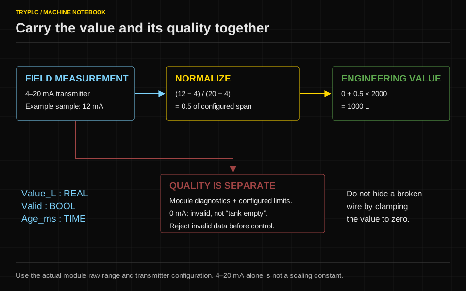
Do the arithmetic before opening the software: low endpoint, midpoint, high endpoint. Then test a disconnected or diagnostically invalid signal. A conversion that produces the correct midpoint but presents a broken loop as an empty tank is not ready for control. Units and validity travel with the value all the way to the decision.

The number is the end of a measurement chain

A pressure transmitter sends 12 mA to an input module. Your program displays 5.0 bar. That looks reasonable for a 0–10 bar instrument. Before trusting it, trace the chain: pressure reaches a sensing element; the transmitter turns that into current; the module samples the current; the driver supplies a number and diagnostics; your program converts the number into an engineering value.

Every link can be wrong independently. A transmitter configured for 0–16 bar will still send a believable current. A module configured for 0–20 mA will still produce a changing number. A program using the wrong endpoint can still display a smooth trend. Smooth is not the same as correct.

Begin the signal specification with the instrument tag, engineering range, electrical range, module configuration, raw representation and failure response. Put those facts beside the I/O list. Scaling belongs to this boundary, before a sequence or controller consumes the measurement.

Work the conversion forward and backward

For a linear transmitter mapping 0–10 bar onto 4–20 mA:

fraction = (current_mA - 4) / (20 - 4)
pressure_bar = 0 + fraction × (10 - 0)

At 12 mA: fraction = 8 / 16 = 0.5
pressure = 5 bar

The general formula works for other endpoints:

engineering = engLow
            + (raw - rawLow) × (engHigh - engLow)
              / (rawHigh - rawLow)

Here, rawLow and rawHigh are the values the configured module reports at the electrical endpoints. They are not necessarily 4 and 20. Do not subtract four from a raw integer just because the transmitter uses four milliamps.

Manufacturers use different representations, sometimes with choices on the same device. Beckhoff's EP31xx documentation, for example, includes a configuration mapping 4–20 mA to 0–32767. Other ranges and products differ. Use the table for the actual module and configuration. Check the manufacturer's representation table.

Test the inverse as well. If the HMI shows 7.5 bar, this transmitter should be near 16 mA. That prediction gives a technician an independent comparison rather than a second display of the same faulty calculation.

A defensible scaling boundary

This ST body excerpt assumes endpoints and the raw input are already converted to REAL. Diagnostics come from the configured input channel. It does not hardcode a universal wire-break threshold.

ConfigurationValid := (RawHigh > RawLow) AND (EngHigh > EngLow);
MeasurementValid := ConfigurationValid
    AND ChannelHealthy
    AND SampleFresh;

IF MeasurementValid THEN
    UnclampedValue := EngLow
        + (RawValue - RawLow)
        * (EngHigh - EngLow) / (RawHigh - RawLow);
    BelowNominal := UnclampedValue < EngLow;
    AboveNominal := UnclampedValue > EngHigh;
    DisplayValue := LIMIT(EngLow, UnclampedValue, EngHigh);
ELSE
    BelowNominal := FALSE;
    AboveNominal := FALSE;
END_IF;

The example accepts increasing raw and engineering ranges. An application supporting reversed engineering ranges needs different validation and nominal-limit logic. The purpose is to expose assumptions, not hide them in a clever universal formula.

Keep UnclampedValue for diagnosis. A clamped display can be useful for drawing a bar inside its frame, but clamping must not make a failed input look healthy. When invalid, the last numeric value remains in this excerpt; every consumer must also use MeasurementValid. The HMI should show a stale or invalid indication rather than quietly holding a believable number.

Resolution is not accuracy

Suppose an illustrative converter has 4,096 possible codes spanning 0–100 bar, including both endpoints. Adjacent codes differ by about 100 / 4095 = 0.0244 bar. Displaying six decimal places does not recover pressure information that was never measured.

Accuracy includes other effects: sensor error, calibration, wiring, electrical noise and temperature influences. Resolution describes available numeric steps. A high-resolution measurement can be consistently wrong. A more accurate instrument can still show a small staircase in a slow trend.

For a practical decision, compare the entire measurement uncertainty with the process tolerance. If the allowed filling error is smaller than the uncertainty of the measurement chain, no amount of ST formatting will rescue the design. The instrument, mechanical arrangement or acceptance requirement needs review.

Filter noise without hiding the event

A simple first-order filter updates a displayed value by a fraction of the difference:

filteredNext = filteredNow + alpha × (measured - filteredNow)
alpha = dt / (tau + dt)

For a 0.1-second sample interval and a 0.9-second time constant, alpha is 0.1. A step from zero to ten produces filtered samples of 1.0, 1.9 and 2.71. The calmer display is also slower. That delay may be fine for an operator trend and unsuitable for a fast jam detector.

Document which value each decision uses. Keep raw, scaled and filtered signals distinguishable. If a measurement becomes invalid, decide whether the filter holds, resets or tracks a substitute. On recovery, a filter starting far from reality can delay control again. A simple simulation should let you add noise, break the wire and restore it while observing both validity and filtered output.

Decide what a failed sensor means

For a cooling-water temperature display, a bad sensor might simply mark a maintenance condition. For a dosing operation whose stop decision depends on the measurement, invalidity may require an immediate process hold. Neither response is universal.

Write a small decision table: invalid before start, invalid during operation, recovered after a short outage, recovered after a long outage. Include who may authorise continuation and what material must be checked. An ordinary process hold is not a certified protective function; any hazardous condition requires its separately engineered protection.

Try it

A level instrument is ranged 0–2 metres and sends 4–20 mA. At 1.5 metres the module reports 24,575 using a configured 0–32767 raw span. The tank is a vertical rectangular vessel with a 1.2 by 0.8 metre base. Calculate the level and volume. Then explain why using the same volume formula for a horizontal cylindrical tank would be wrong.

Work through the answer

The raw fraction is approximately 24575 / 32767 = 0.75. Level is therefore about 1.5 metres. Base area is 1.2 × 0.8 = 0.96 square metres. Volume is 0.96 × 1.5 = 1.44 cubic metres, or approximately 1,440 litres. Small differences in the final decimal follow from raw quantisation.

A horizontal cylinder does not contain equal volume in equal height increments. Its cross-sectional width changes with height, so a straight level-to-volume multiplier misstates the inventory. Use the vessel's validated geometry or calibration table. The electrical conversion may be perfectly linear while the physical quantity you ultimately need is not. That distinction prevents a very common commissioning argument about which “scaling” is wrong.