Control a continuous process

Before tuning, ask three questions: does increasing the output raise or lower the measurement, how long before a change becomes visible, and what happens when the request reaches its limit? Wrong control direction cannot be repaired by choosing a smaller gain. A disconnected measurement cannot be repaired by choosing a longer integral time.

First ask which way the process moves

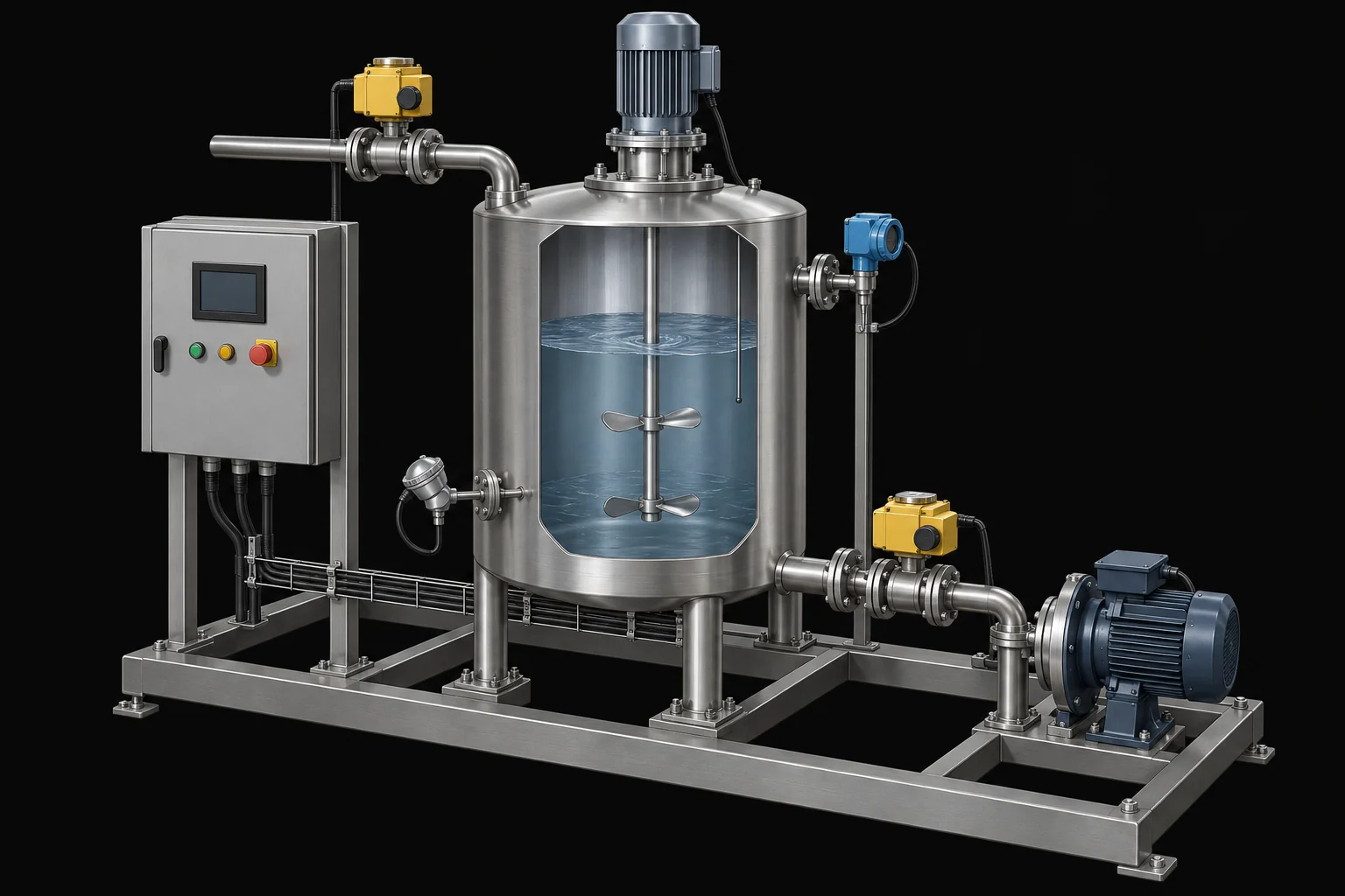
A tank loses water to production. Your PLC can adjust an inlet valve. The request says, “Keep the level at 60%.” A sequence alone cannot decide a fixed valve position because the outlet demand changes. You need feedback: measure the result, compare it with the target, and adjust the input.

Before choosing gains, answer a physical question. If valve command increases, does level eventually rise or fall? Trace the actual installation, including whether the valve is air-to-open, how its positioner interprets the signal, and what the actuator does when supply is lost. A controller with the wrong direction drives an error away from the target with impressive confidence.

For this chapter, more command means more inlet flow. The example is a teaching model, not a tuning prescription for an operating plant. Real commissioning requires an authorised test plan and defined process limits.

Give the process a simple model

For a tank with constant cross-sectional area:

change in volume = (inlet flow - outlet flow) × elapsed time
change in level = change in volume / tank area

Take a one-square-metre tank. Inlet flow is 0.012 cubic metres per second and outlet flow is 0.010. The net 0.002 cubic metres per second raises the level by 0.002 metres per second. In ten seconds, level increases by 20 millimetres.

This calculation explains something a gain table cannot: a tank integrates imbalance. If inlet equals outlet, the level stops changing wherever it currently is. It does not automatically return to the setpoint. For temperature, the model would include stored heat, heat transfer and losses. For pressure, compressibility and restrictions matter. Match your intuition to the process you have.

What the three PID letters contribute

Proportional action responds to current error. With error = setpoint - measured, a gain of 2 percentage points of valve opening per level percentage point produces a 10-point output change for a 5-point error. Specify units; “gain 2” alone leaves too much unstated.

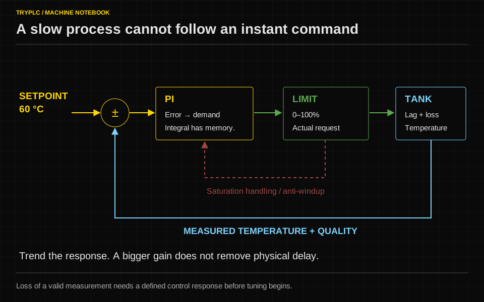
Integral action accumulates error over time. It can supply the steady command needed to balance a disturbance while the measured value reaches its target. That accumulated contribution is memory, so mode changes and output limits matter.

Derivative action responds to rate of change. It can help some processes anticipate movement, but it also responds to measurement noise. Many practical loops use PI rather than all three terms. The right choice follows the process and the vendor block's formulation, not an obligation to use every feature.

Vendor blocks may use different parameter conventions: integral time versus integral gain, proportional band versus proportional gain, derivative on error versus measurement. Copying numbers between blocks without converting those meanings is not a tuning method.

A small numerical controller you can inspect

The following equations describe a simplified discrete PI teaching model with output in percent. They are not a complete production controller:

error = target - measurement
proportional = Kp × error
candidateIntegral = integral + Ki × error × dt
candidateOutput = bias + proportional + candidateIntegral
output = clamp(candidateOutput, 0, 100)

Suppose bias is 40%, proportional contribution is 10%, and integral is 5%. Output is 55%. If the valve is stuck at 30% actual opening, the PLC can continue requesting more while nothing useful changes. A trend of command alone hides that failure. Add measured position or process-response evidence where the equipment provides it.

Run the calculation at a known interval and give the block the correct interval. Doubling the frequency while keeping an incorrect dt doubles the accumulated integral action per real second. Calling a controller conditionally can also make the effective sampling interval unpredictable.

Why an integrator needs an escape route

Imagine the tank starts low while the inlet valve is already fully open. Positive error keeps adding to the integral. After the tank finally reaches the target, that stored contribution may keep the valve open and cause overshoot. This is integral windup.

One teaching strategy rejects an integral update that would push an already limited output farther into the limit, while allowing an update that brings it back. Production blocks may use tracking or other anti-windup mechanisms. Beckhoff documents an example that limits integral accumulation at output bounds while permitting movement back toward the allowed range. Inspect an actual anti-windup implementation.

The real actuator may have additional limits. If downstream logic reduces the requested output, the controller should know the effective output through its supported tracking mechanism. Otherwise its internal picture and the valve's actual command diverge.

Manual mode should not leave a surprise waiting

An operator takes manual control and holds the valve at 35%. The automatic controller still contains a 90% demand. Switching directly back to automatic produces a jump, even though the operator never asked for one.

“Bumpless transfer” means arranging the controller's internal state so the transfer itself does not cause an unnecessary output step. In the simple PI model, track the integral toward manualOutput - bias - proportional while manual is active. Real controllers offer dedicated manual, tracking and initialisation inputs; use their documented behaviour. Also decide whether the setpoint tracks the process in manual or keeps the operator's chosen target. Those choices affect what happens immediately after transfer.

Do not promise perfect smoothness under every circumstance. If a process constraint changes at the same time, an output change may be necessary. The important distinction is whether the change follows the control requirement or merely exposes stale internal memory.

Read trends as evidence

Trend setpoint, measurement, requested output, effective output and mode on a common time axis. Add validity and saturation indications. A flat 100% output with a falling temperature may mean insufficient heating capacity, an open contactor, wrong direction, or a failed measurement. Increasing gain cannot distinguish them.

Change one thing at a time during a controlled test. Record the initial condition, disturbance, settings and observed response. Your aim is not the most dramatic trace. It is acceptable settling, overshoot and disturbance rejection within the real process constraints.

Try it

A heater is in manual at 25%. Its PI controller calculates a proportional contribution of 12% and uses zero bias. What integral contribution gives a smooth transfer at that instant? Then the temperature sensor becomes invalid. Should the controller continue using its last measurement indefinitely?

Work through the answer

Set the tracked integral contribution to 25 - 12 = 13%. The automatic sum then equals the current manual output. That arithmetic illustrates the principle; implement it through the selected block's supported tracking interface rather than modifying hidden internals.

Continuing indefinitely with a stale measurement turns feedback control into an unacknowledged open-loop command. Define an invalid-measurement response based on the process: inhibit heating, enter a controlled hold, or use an independently justified substitute. Report the reason and require the agreed recovery action. The controller handles normal regulation; independent protection handles hazards. In Analog signals and scaling, validity travelled with the value. Here you see why that extra Boolean matters.